Introduction

    At the beginning of this year, a technical club at my university hosted a "Build an AI/ML model" workshop aimed towards teaching freshers how to get started with AI. The workshop involved building a digit classification model that recognised handwritten digits using TensorFlow on Jupyter notebooks. Although it was a great beginners tutorial on TensorFlow, I felt dissatisfied with that because it didn't explain how the model actually "learnt", improving its weights and reducing the loss function.

    As much I'd like to go into detail about every part of the code line by line like my previous blog, it would be simply too cumbersome for my liking as a.) The code is relatively bigger, and b.) I find the mathematics behind it more fascinating. Additionally, I would highly suggest reading this textbook by Michael Nielsen to have a more thorough understanding.

Neurons

The foundation of any neural network, whether biological or artificial, lies in its basic building blocks: neurons. In the human brain, neurons are specialized cells that transmit information through electrical and chemical signals. They form complex networks that enable us to think, learn, and perform various cognitive tasks. Similarly, in the realm of artificial intelligence, neurons are the computational units that process and transmit data within a network, enabling the system to learn and make decisions.

    When we talk about artificial neurons, we're referring to mathematical functions that receive one or more inputs, process them, and produce an output. These artificial neurons are designed to mimic the behavior of their biological counterparts, albeit in a much simpler and more abstract form.

Perceptron

    Similar to the neurons in your brain, computer neurons re-emit signals recieved from other sources. Perhaps the simplest form of a computer neuron would be a perceptron.

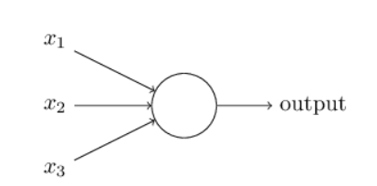
A perceptron takes in one or more binary inputs (0/1) and outputs one binary value. It is calculated by

$$ output = \begin{cases} 0 & \text{if } \sum_j w_j x_j \leq \text{threshold} \newline 1 & \text{if } \sum_j w_j x_j > \text{threshold} \end{cases} \tag{1} $$

or converting $\sum_j w_j x_j$ to its dot product forms $w \cdot x$ and re-defining the threshold as the convention, bias $b$, we can rewrite it as

$$ output = \begin{cases} 0 & \text{if } w \cdot x - b \leq 0 \newline 1 & \text{if } w \cdot x - b > 0 \end{cases} \tag{2} $$

That's the basic mathematical model. It says yes or no depending on how the inputs are formed, A simple example would be: imagine your friends call you for a weekend getaway at the beach. Your decision to go depends on three factors:

1. Is your boyfriend/girlfriend joining?
2. Is it going to rain?
3. Are you going by car?\end

• You place option 1 as the most important, and weigh that in at $w_1 = 3$
• You weigh in option 2 at $w_2 = 2$ and
• $w_3 = 1$

$x_i$ basically means "is option $i$ true or not, if it is $x_i = 1$ else its $0$. Assuming a bias $b = 5$.

if option 1, 3 are true and 2 is false:

$$w \cdot x - b = (3×1)+(2×0)+(1×1)= -1 < 0$$ so you don't go but if all 3 are true:

$$w\cdot x−b=(3×1)+(2×1)+(1×1)−5=3+2+1−5=1>0$$

So, you decide to go.

    This example illustrates how a perceptron can make simple decisions based on weighted inputs and a bias. Each weight represents the importance of a corresponding input, and the bias adjusts the threshold for decision-making. By adjusting the weights and bias, a perceptron can be trained to perform various logical operations and make decisions based on input data.

Sigmoid Neuron

    To see how learning might work, suppose we make a small change in some weight (or bias) in the network. What we'd like is for this small change in weight to cause only a small corresponding change in the output from the network. Schematically, here's what we want (sort of):

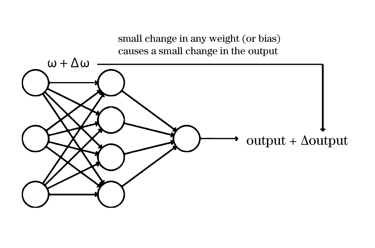
If a small change in a weight (or bias) causes a small change in the output, we can adjust the weights and biases to improve the network's performance. For example, if the network incorrectly classifies an image as an "8" instead of a "9", we can slightly change the weights and biases to make the network more likely to classify the image as a "9".

    Unfortunately for our perceptrons, a small change in the weights or bias of one of them in the network can sometimes switch the output of the perceptron from 1 to 0 and vice versa. That flip may then cause the behaviour of the rest of the network to completely change in some very complicated way. So while your "9" might now be classified correctly, the behaviour of the network on all the other images is likely to have completely changed in some hard-to-control way.

The solution to this was a new, but similar type of neuron called the sigmoid neuron. Which works with this logic:

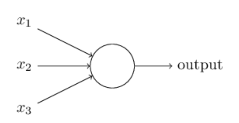
It looks the same as the perceptrons that we saw earlier. Altho it has a few changes:

1. Instead of the inputs being 0 or 1, these inputs can take on any value between 0 and 1, eg: 0.532... could be one input.
2. Just like a perceptron, it has weights for each input $w1, w2...$ and bias b. But the output is not 0 or 1. Its $\sigma(w \cdot x + b)$ where the sigma function (also called the logistic function) is:

$$ \sigma(z) = \frac{1}{1 + e^{-z}} \tag{3}$$

    At first it looks a lot more complicated than the perceptron but suppose $z≡w⋅x+b$ is a large positive number. Then $e−z≈0$ and so $σ(z)≈1$. In other words, when $z=w⋅x+b$ is large and positive, the output from the sigmoid neuron is approximately 1, just as it would have been for a perceptron. Suppose on the other hand that $z=w⋅x+b$ is very negative. Then $e−z→∞$, and $σ(z)≈0$. So when z=w⋅x+b is very negative, the behaviour of a sigmoid neuron also closely approximates a perceptron.

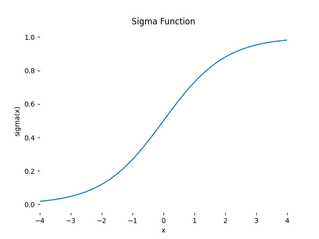
So basically a sigma function is a smoother version of the step function. Which allows us to make slight changes in $w$ and $b$ for slight change in the output. As approximated by:

$$ \Delta \text{output} \approx \sum_j \frac{\partial \text{output}}{\partial w_j} \Delta w_j + \frac{\partial \text{output}}{\partial b} \Delta b \tag{4} $$

    This can be useful, for example, if we want to use the output value to represent the average intensity of the pixels in an image input to a neural network. But sometimes it can be a nuisance. Suppose we want the output from the network to indicate either "the input image is a 9" or "the input image is not a 9". Obviously, it'd be easiest to do this if the output was a 0 or a 1, as in a perceptron. But in practice we can set up a convention to deal with this, for example, by deciding to interpret any output of at least 0.5 as indicating a "9", and any output less than 0.5 as indicating "not a 9".

The architecture of neural networks

Suppose we have the network:

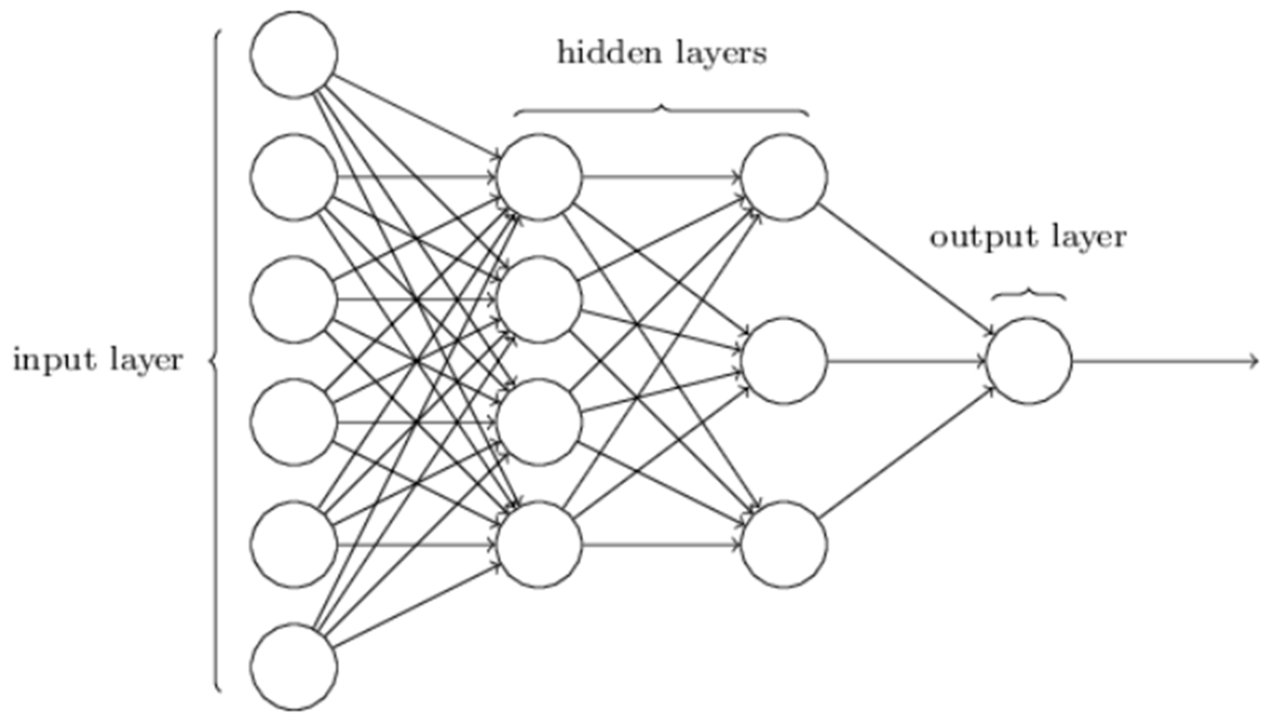
The leftmost layer in this network is called the input layer, and the neurons within the layer are called input neurons. The rightmost or output layer contains the output neurons, or, as in this case, a single output neuron. The 2 middle layers are called hidden layers, called because the neurons in these layers are neither inputs nor outputs.

    Up to now, we've been discussing neural networks where the output from one layer is used as input to the next layer. Such networks are called feedforward neural networks. This means there are no loops in the network - information is always passed forward, never passed back. If we did have loops, we'd end up with situations where the input to the σ function depended on the output. That'd be hard to make sense of, and so we'll keep it outside the scope of this blog.

    However, There are artificial neural networks that make sense of the loops called recurrent neural networks. The idea of which is allowing neurons to fire only a few times or a fixed duration.

    Our program will solve the problem of classifying individual digits and not a string of numbers. To recognize individual digits we will use a three-layer neural network:

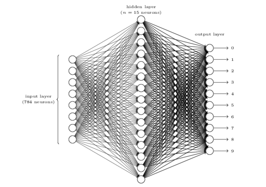
Our training data for the network will consist of many $28$ by $28$ pixel images of scanned handwritten digits, and so the input layer contains $784=28×28$ neurons. The input pixels are greyscale, with a value of $0.0$ representing white, a value of $1.0$ representing black, and in between values representing gradually darkening shades of grey.

    The second layer of the network is a hidden layer. We denote the number of neurons in this hidden layer by $n$, and we'll experiment with different values for $n$. The example shown illustrates a small hidden layer, containing just $n=15$ neurons.

    The output layer of the network contains 10 neurons. If the first neuron fires, i.e., has an output $≈1$, then that will indicate that the network thinks the digit is a $0$. If the second neuron fires then that will indicate that the network thinks the digit is a $1$. And so on.

    A Computer Science perspective might wonder why we use 10 output neurons. After all, the goal of the network is to tell us which digit $(0,1,2,…,9)$ corresponds to the input image. A seemingly natural way of doing that is to use just $4$ output neurons, treating each neuron as taking on a binary value, depending on whether the neuron's output is closer to 0 or to 1. Four neurons are enough to encode the answer, since $2^4=16$ is more than the 10 possible values for the input digit. Why should our network use 10 neurons instead? Isn't that inefficient?

    This was my initial thought and turns out; one could implement a 4 output-neuron architecture, but the hidden layers seem to struggle with selecting features and they find 10 neurons simpler to push their outputs to. Although this is all just a heuristic, and people are free to try out different architectures just to play around.

Learning with gradient descent

We'll use the notation $x$ to denote a training input. It'll be convenient to regard each training input $x$ as a $28×28=784$-dimensional vector. Each vector input represents the grey value from $0$ to $1$ for each pixel. For example, if a particular training image, $x$, depicts a $6$, then $y(x)=(0,0,0,0,0,0,1,0,0,0)^T$ is the desired output from the network.

    In order to quantify how correct the model is we could introduce a "cost" function (also called as loss function). Similar to how your teacher gives you varying amount of marks on a answer depending on how correct it is. This function allows us to determine how correct the model is and how confident it gives its results.

$$C(w,b) = {\frac1 {2n}} \sum_x ||y(x) - a||^2 \tag{5}$$

This equation is called $mean \space squared \space error$ or a quadratic cost function. Here,

   $\bullet$ $w$ denotes the collection of all weights in the network,

   $\bullet$ $b$ all the biases, $n$ is the number of training inputs,

   $\bullet$ $a$ is the vector of outputs from the network when $x$ is input, and the sum is over
    all training inputs, $x$.

   Of course, the output a depends on $x$, $w$ and $b$, but to keep the notation simple I haven't explicitly indicated this dependence. The notation $∥v∥$ just denotes the usual length function for a vector $v$.

    The model has done a good job if it can find weights and biases so that $C(w,b)≈0$. By contrast, it's not doing so well when $C(w,b)$ is large - that would mean that $y(x)$ is not close to the output a for a large number of inputs. So the aim of our training algorithm will be to minimize the cost $C(w,b)$ as a function of the weights and biases. We'll minimize it using a method called gradient descent.

for a given cost function $C$ with parameters $v1$ and $v2$, the change in $C$ caused by changes in $v1$ and $v2$ is given by:

$$\Delta C \approx \frac{\partial C}{\partial v_1}\Delta v_1 + \frac{\partial C}{\partial v_2}\Delta v_2$$

We have to choose $\Delta v_1$ and $\Delta v_2$ such that $\Delta C$ turns out to be negative as to allow for the function to descend.

We'll denote the gradient vector by $∇C$, i.e.:

$$\nabla C \equiv \left(\frac{\partial C}{\partial v_1}, \frac{\partial C}{\partial v_2}\right)^T$$

With these definitions, the expression for $ΔC$ can be rewritten as

$$\Delta C \approx \nabla C \cdot \Delta v $$

This equation allows us to choose Δv in a way so as to make ΔC negative. In particular, suppose we choose

$$Δv=−η∇C$$

Where $η$ is a small, positive number (also called as learning rate).

$$ΔC≈−η∇C⋅∇C=−η∥∇C∥^2$$

Because $∥∇C∥2≥0$, this guarantees that $ΔC≤0$, i.e., $C$ will always decrease, never increase.

$$\therefore v→v'=v−η∇C \tag{6}$$

If we keep doing this, over and over, we'll keep decreasing $C$ until we reach (or get close to) a global minimum.

    You can think of this update rule as defining the gradient descent algorithm. It gives us a way of repeatedly changing the position v in order to find a minimum of the function $C$. The rule doesn't always work - several things can go wrong and prevent gradient descent from finding the global minimum of $C$. But, in practice gradient descent often works extremely well.

How can we apply gradient descent to learn in a neural network? The idea is to use gradient descent to find the weights $w_k$ and biases $b_l$ which minimize the cost.

$$w'_k = w_k - \eta \frac{\partial C}{\partial w_k}$$ $$b'_l = b_l - \eta \frac{\partial C}{\partial b_l}$$

    An idea called stochastic gradient descent can be used to speed up learning. The idea is to estimate the gradient $∇C$ by computing $∇C_x$ for a 'mini batch' of a small sample of randomly chosen training inputs. By averaging over this small sample it turns out that we can quickly get a good estimate of the true gradient $∇C$, and this helps speed up gradient descent, and thus learning.

    We pick a randomly chosen mini-batch of training inputs and train the model. We pick out another randomly chosen mini-batch and train with those. And so on, until we've exhausted the training inputs, which is said to complete an epoch of training. At that point we start over with a new training epoch.

    We can think of stochastic gradient descent as being like political polling: it's much easier to sample a small mini-batch than it is to apply gradient descent to the full batch, just as carrying out a poll is easier than running a full election.

All this information until now should be enough for implementing the classification model. An implementation in python is written below with numpy.

The code

You can run a copy of it in your local machine (I tried it on a linux machine with 16gb of ram with no GPU). You might find some problems with importing keras.datasets, you could replace it with from tensorflow.keras.datasets import mnist (or even manually download it into your machine) as per your convenience.

    Note that this model generates ~75% accuracy (better than 10% from random guessing) and is not at all production ready, but is a very very simplified version with only sigmoid-activation functions (compared to Rectifiers and softmax activations) for educational purposes.

import pandas as pd
import numpy as np
import pickle
from keras.datasets import mnist
import matplotlib.pyplot as plt

def sigmoid(Z):
    return 1 / (1 + np.exp(-Z))

def derivative_sigmoid(Z):
    sig = sigmoid(Z)
    return sig * (1 - sig)

def init_params(size):
    W1 = np.random.rand(10,size) - 0.5
    b1 = np.random.rand(10,1) - 0.5
    W2 = np.random.rand(10,10) - 0.5
    b2 = np.random.rand(10,1) - 0.5
    return W1,b1,W2,b2

def forward_propagation(X,W1,b1,W2,b2):
    Z1 = W1.dot(X) + b1 
    A1 = sigmoid(Z1) 
    Z2 = W2.dot(A1) + b2
    A2 = sigmoid(Z2)
    return Z1, A1, Z2, A2

def mse_loss(A2, Y, m):
    Y_one_hot = np.identity(A2.shape[0])[Y].T 
    return np.mean(np.sum((A2 - Y_one_hot)**2, axis=0))

def backward_propagation(X, Y, A1, A2, W2, Z1, m):
    Y_one_hot = np.identity(A2.shape[0])[Y].T 
    dZ2 = 2 * (A2 - Y_one_hot) / m
    dW2 = dZ2.dot(A1.T)
    db2 = np.sum(dZ2, axis=1, keepdims=True)
    dZ1 = W2.T.dot(dZ2) * derivative_sigmoid(Z1)
    dW1 = dZ1.dot(X.T)
    db1 = np.sum(dZ1, axis=1, keepdims=True)
    return dW1, db1, dW2, db2

def update_params(alpha, W1, b1, W2, b2, dW1, db1, dW2, db2):
    W1 -= alpha * dW1
    b1 -= alpha * np.reshape(db1, (10,1))
    W2 -= alpha * dW2
    b2 -= alpha * np.reshape(db2, (10,1))

    return W1, b1, W2, b2

def get_predictions(A2):
    return np.argmax(A2, 0)

def get_accuracy(predictions, Y):
    return np.sum(predictions == Y)/Y.size

def gradient_descent(X, Y, alpha, iterations):
    size, m = X.shape
    W1, b1, W2, b2 = init_params(size)

    for i in range(iterations):
        Z1, A1, Z2, A2 = forward_propagation(X, W1, b1, W2, b2)
        dW1, db1, dW2, db2 = backward_propagation(X, Y, A1, A2, W2, Z1, m)
        W1, b1, W2, b2 = update_params(alpha, W1, b1, W2, b2, dW1, db1, dW2, db2)
        
        if (i+1) % int(iterations/10) == 0:
            print(f"Iteration: {i+1} / {iterations}")
            prediction = get_predictions(A2)
            print(f'Accuracy: {get_accuracy(prediction, Y):.3%}')
            print(f'MSE Loss: {mse_loss(A2, Y, m):.4f}')
    return W1, b1, W2, b2

def make_predictions(X, W1 ,b1, W2, b2):
    _, _, _, A2 = forward_propagation(X, W1, b1, W2, b2)
    predictions = get_predictions(A2)
    return predictions

def show_prediction(index,X, Y, W1, b1, W2, b2):
   # None => creates a new axis of dimension 1, this has the effect of transposing X[:,index] which is an np.array of dimension 1 (row) and which becomes a vector (column)
     # which corresponds to what is requested by make_predictions which expects a matrix whose columns are the pixels of the image, there we give a single column
    vect_X = X[:, index,None]
    prediction = make_predictions(vect_X, W1, b1, W2, b2)
    label = Y[index]
    print("Prediction: ", prediction)
    print("Label: ", label)

    current_image = vect_X.reshape((WIDTH, HEIGHT)) * SCALE_FACTOR

    plt.gray()
    plt.imshow(current_image, interpolation='nearest')
    plt.show()

#MAIN

(X_train, Y_train), (X_test, Y_test) = mnist.load_data()
SCALE_FACTOR = 255 # to prevent overflow on exp();
WIDTH = X_train.shape[1]
HEIGHT = X_train.shape[2]

X_train = X_train.reshape(X_train.shape[0],WIDTH*HEIGHT).T / SCALE_FACTOR
X_test = X_test.reshape(X_test.shape[0],WIDTH*HEIGHT).T  / SCALE_FACTOR

W1, b1, W2, b2 = gradient_descent(X_train, Y_train, 0.25, 200)

with open("trained_params.pkl","wb") as dump_file:
    pickle.dump((W1, b1, W2, b2),dump_file)

with open("trained_params.pkl","rb") as dump_file:
    W1, b1, W2, b2=pickle.load(dump_file)

show_prediction(0,X_test, Y_test, W1, b1, W2, b2)
show_prediction(1,X_test, Y_test, W1, b1, W2, b2)
show_prediction(2,X_test, Y_test, W1, b1, W2, b2)
show_prediction(100,X_test, Y_test, W1, b1, W2, b2)
show_prediction(200,X_test, Y_test, W1, b1, W2, b2)